Basic

This is a warmup question to kick off a conversation, there is no right or wrong as long as you pick an algorithm that you know ins and outs when the interviewer dives deep into details.

Sample answer:

Thank you, that's a very interesting question, my favorite machine learning algorithm is Random Forest because of its ease of use and high performance.

1. Based on my past experience in building machine learning models, Random Forest has consistently generated good results in both classification and regression problems;

2. Random Forest also trains very fast without a lot of feature engineering, which saves a lot of time and allowed me to build a quick prototype and communicate my results to the business;

3. Because Random Forest randomly samples the training data and variables, it is less prone to outliers and over-fitting.

4. Lastly, RF also has some bells and whistles such as giving us an idea of how important each variable is, which makes it easy for us to explore the data and intuitively validate our understanding of the data.

N-fold cross-validation is a re-sampling technique, commonly used to evaluate a machine learning model's performance.

The raw data set is randomly partitioned into n disjoint subsets, and one of the subsets is used as the testing data, while the rest is used as the training data for modeling.

The process is repeated n times and the performance metrics such as accuracy are aggregated by taking the average of the n accuracies.

A common value of n is 5, so that 80% of the samples are used in training, and 20% for testing.

Over-fitting happens when a machine learning model "tries too hard" to make a perfect prediction on training data.

For example, a single decision tree developed many levels and try to predict a perfect label for every single data point, and every decision block (leave) has only one sample.

A typical over-fitting pattern can be detected by re-apply the model to a hold-out sample, and if the performance on the holdout sample is quite different than its performance on the training data.

It most likely is an over-fitted model, which means the model won't generalize well.

For example: in linear regression models, we can use regularization such as L1 (Lasso) or L2 (Ridge) methods to help shrink or reduce the impact of too many parameters.

For a decision tree, we can create a large tree (with many depths), and use cross-validation to prune the tree back to avoid over-fitting.

For a neural network, dropout is an effective way to help avoid over-fitting.

Generally speaking, in practice, there are two ways to deal with missing values.

1. Skip those samples

If there is no evidence that the missing of certain fields is not random, and the number of rows/samples with missing data is only a small percentage of your training data, you can safely remove those samples.

If there is a strong correlation with samples that has a missing value to other variables, e.g., in a survey people who earn less than 50k per year may feel uncomfortable sharing their income bucket information.

Instead of removing all those samples (which introduces sample bias, and your training data is no longer a good representation of the overall population), we can keep those rows but fill the missing income bucket variables with a new value of "missing".

2. Imputation

If the missing values are random, no strong correlation between missing values and other variables, we can replace the missing values using the maximum likelihood philosophy.

For example, we can fill the median value for continuous variables, or the most common non-missing value for categorical variables.

When your samples are extremely unbalanced, for example: in a binary classification problem and the ratio of class 1 vs class 2 is 99% vs 1% (like click event prediction for display ads), usually, we can down-sampling the larger group to achieve a 50/50 (or other ratios such as like 70/30 split) ratio for the new training data.

After training the model on the new training data (50/50 of class 1 vs class 2), the key to making sure your upsampling works is to test your model on a hold-out sample without any resampling.

By doing this, you will be able to evaluate the model performance in the real production environment.

Since the hold-out sample has 99% of class 1 data, if you create a dummy predictor and simply predict everything to be class 1, you will still have 99% accuracy.

So, instead of using overall accuracy, we need to change the metric to f1-score, which is the harmonic mean of precision and recall, to make sure the model is a good model.

This is a typical question to test your understanding of the model evaluation process.

The key idea behind the time-sensitive training data is to think about what the real-world data will look like.

e.g., if you are building a time-series model to predict next month's web traffic, you can't use future months' data.

So instead of randomly splitting your raw data into training and testing subsets, you will need to separate them by time. e.g., using the month 1 to month 13 data to train your model, use month 14 to test its performance. 

The main goal of regularization is to help us avoid over-fitting. When the number of variables and the complexity of the model is high, the model can achieve near-perfect performance on the training data, but due to lack of generalization, it will perform poorly for unseen new data.

Regularization helps us reduce the complexity of the model, and avoid 'over-learning' on the training data, so it can perform better on unseen data points.

Theoretical explanation:

The mean squared error can be decomposed into two parts:

The bias part and the variance part. 

Bias:

Variance:

The bias represents how your model performs on the training sample, and the variance is how it will generalize for future unseen samples.

Intuitive explanation 

Imagine if we are shooting a target, the best scenario is that we consistently hit the bullseye.

Chart 1: low bias, low variance (best scenario).

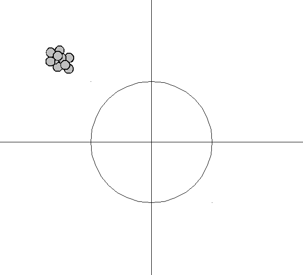
Chart 2: bias high, variance low

If we are consistent but every time we shoot far away from the bullseye, it's the high bias, low variance scenario.

Similarly, we also have low bias, high variance (chart 3) and high bias, high variance scenarios:

Chart 3: bias low, variance high.

Chart 4: bias high, variance high

The most common way to represent categorical features is to use the one-hot encoding method.

SVM means support vector machine, it is a linear algorithm that tries to find the best separation of two classes of samples for a binary classification problem. 

It is formalized as an optimization problem and the goal is to find a line (in 2d) or hyperplane (higher dimensional space) that represents the largest separation, or margin, between the two classes o samples.

The hyperplane that maximizes the margin is called the support vector.

1. Linear;
2. Polynomial;
3. RBF: Radial basis function;
4. Sigmoid

False Positive represents the probability when we mistakenly predict a negative case as a positive case.

False Positive increases the Recall and is usually preferred if the potential loss/penalty is very high.

For example: in extreme weather prediction, we'd rather mistakenly predict the weather as a potential hurricane, than not treat it as a potential risk.

False-negative means we mistakenly predict a positive case as the negative case.

It happens commonly in recruiting, often a company tends to be very strict in making an offer to a candidate so that they won't hire someone who turns out to be a poor employee.

They'd rather reject a qualified candidate rather than accept an unqualified candidate.

The "Naiveness" or "Naivety" in a Naive Bayes algorithm stems from the assumption of conditional independence of every pair of features X given the class variable y, which significantly simplifies the computation, but in a real world, it's rarely true.